The Convolutional Model in the Time Domain
This blog post will review the continual evolution of seismic reflection survey methods and imaging technology since its infancy. The types of data used to characterize the subsurface have grown dramatically over the years. Yet, 3D seismic data remains the primary source of spatial subsurface data used to create complex earth models through methods such as the convolutional model.
At its very foundation, the seismic reflection method was created through integrated scientific collaboration. One of the primary goals of these collaborations is to help engineers efficiently extract hydrocarbons and provide the world with affordable energy. Seismic reflection data surveys are critical to carbon capture and storage, geothermal prospecting, near-surface hazard surveys for wind farms, nuclear installations, and civil engineering and infrastructure. They have improved the quality of life for people globally.
The seismic reflection method aims to understand the physics behind subsurface geology. From the 1920s until the early 1960s, this was simply used to help define structure. However, in 1963, the introduction of digital recording enabled seismic reflection surveys to capture a more defined dynamic range of amplitudes and interpret amplitude variations.
The convolutional model in the time domain permits the creation of accurate subsurface models through seismic data analysis and processing. The convolution theorem says that the Fourier transform of a convolution of two signals is the point-wise product of their Fourier transform under suitable conditions. In this instance, convolution in one domain — time — equals point-wise multiplication in the other domain — frequency.
The concept of the convolutional model in seismic data processing is important to understand the reflectivity of each trace in a 3D seismic volume. Mathematically, the convolutional model in the time domain is given by:
x(t)=ω(t)*e(t)+n(t) (Yilmaz, 2001)
Where:
x(t) is the recorded seismogram
ω(t) is the seismic wavelet
e(t) is the earth’s impulse response or reflectivity series
n(t) is the noise inherent in the recorded seismogram
The convolutional model in the time domain makes it possible to understand the reflectivity of each trace in a 3D seismic volume. The seismic trace is composed of reflectivity convolved with the earth’s response — in other words, a wavelet or seismic trace — plus ambient noise. Removing that noise is required to accurately depict or image the subsurface in a model. Deconvolution breaks down the recorded seismogram into distinct parts.
This approach to seismic reflection data interpretation makes imaging more accurate, allowing teams to account for ambient noise. There are several potentially useful applications for the convolutional model in seismic data processing. For companies looking to drill into new territory, this can provide an accurate model of what exists beneath the surface.
The following graph depicts the model in action.
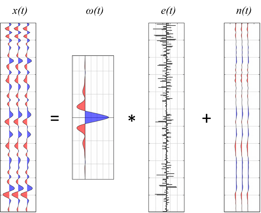
The recorded seismogram is characterized by convolving the seismic wavelet with the earth’s reflectivity series and adding the inherent ambient noise. For simplicity, this concept is illustrated using a stacked seismic trace, a wavelet generated from 3D seismic data, a reflectivity series generated by sonic and density well logs, and noise represented as the difference between the seismic and synthetic traces.
References:
Yilmaz, O. (2001). Seismic Data Analysis: Processing, Inversion, and Interpretation of Seismic Data (2 ed., Vol. 1). (M. R. Cooper, Ed.) Tulsa, Oklahoma, USA: Society of Exploration Geophysics. doi:http://dx.doi.org/10.1190/1.97...
Post Date
Apr 12, 2023Post Category
Technical Papers
Author
Andrew Lewis