Delaware Basin Fill Zone Revealed for the First Time Ever: How HTD Field Test Uncovered the Geologic Near-Surface Mysteries Hiding the Richest Unconventional Resource Play in the World

Bruce Karr, Andrew Lewis, Stephen Klug and Mike Henry (Fairfield Geotechnologies)

Lin Zheng, Shuang Sun (Viridien)

Summary

The Permian Basin is the most prolific unconventional oil and gas basin in the world. Even within the greater Permian Basin, the Delaware Basin (DB), compared to the Midland Basin, has the greatest stacked pay reserves. However, within the DB there are two significant seismic challenges: the fill zone and the high velocity near-surface anhydrites. In most cases both geologic challenges have relegated seismic almost negligible for the unconventional lateral drilling underneath the fill zone. The New Mexico Cedar Canyon 3D was designed to resolve this near-surface geology. However, there were many who thought the trace density and source effort were not dense enough, especially in deeper fill, and wanted to add an ultra-high trace density 3D field test. The evolution of this field test study began with tighter source and receiver spatial sampling and ultimately included five different types of receivers and three different amounts of source effort. The result was the revealing of the structural complex near-surface geology and the seismic trace density required to image shallow geology.

Introduction

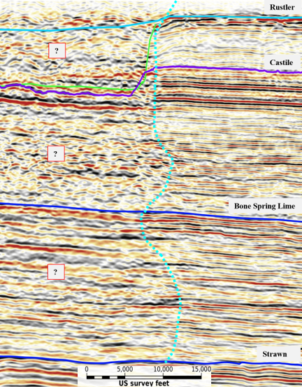
The fill zone in the Delaware Basin covers over 2000 square miles. The importance of resolving the image below the fill zone becomes apparent when billions of barrels of oil are at stake. The legacy PSDM data example (Figure 1) shows how seismic data degrades transitioning into the fill zone. The latest attempt to solve the near-surface geologic challenges is using high trace density (HTD) acquisition survey design (Karr, Lewis, & Bianco, 2021).

The new HTD production survey was designed to image the Rustler formation. The field test led to the discovery of the slow fill and fast fill above the Rustler and further delineation of the Rustler formation. The increased seismic detail showed the Salado collapse zones, Castile anhydrite with salt layers, and illustrated many of the historical reasons why imaging the deeper zones was difficult or impossible.

The Cedar Canyon production survey required approximately 70,000 channels (49,152 live, 18,432 rolling with the spread). The final processed bin size was 41.25ft x 41.25ft with nominal fold of 2048. The production survey covered 72 square miles. The inserted field fill test covered a simple 4 square miles focused on the first 2,500ft of near-surface geology. The key horizon to image was the top of the Rustler with a depth range between 500ft to 1200ft.

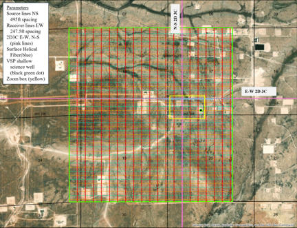
The field test used an additional 35,840 channels. This provided a chance to not only solve the near-surface geology but to compare several receiver types and source effort. The 2816 production channels inside the 4 square mile field test were a string of three 10Hz geophones. An additional 11,008 5Hz geophones were spaced at half the line spacing and half the station spacing. A third set of receivers halved the station spacing again and required another 22,016 channels. For good measure, two 2D3C lines of 10Hz geophones were acquired going through the approximate center of the 4 square mile test area.

The field test used an additional 35,840 channels. This provided a chance to not only solve the near-surface geology but to compare several receiver types and source effort. The 2816 production channels inside the 4 square mile field test were a string of three 10Hz geophones. An additional 11,008 5Hz geophones were spaced at half the line spacing and half the station spacing. A third set of receivers halved the station spacing again and required another 22,016 channels. For good measure, two 2D3C lines of 10Hz geophones were acquired going through the approximate center of the 4 square mile test area.

This provided a single location of reciprocal cross-spreads of 3C geophones to analyze noise and shear wave signal. In addition, a test well was drilled 4600ft with an accompanying VSP using both 3C geophones and vertical fiber recording to the surface. Finally, a buried surface helical fiber 3000ft long overlapping a portion of the east- west 2D3C seismic line was added (Hall, Lawton, & Innanen, 2022).

Field Test Objectives and Design

The main objective was to find the top of the Rustler formation and understand the related decline in data quality while transitioning into the fill. The usual theories of signal/noise, absorption, lack of energy, aliasing, etc., were thought to be the primary problem. However, results derived from recent well drilling, pointed to scattering off a complex shallow Rustler formation as the cause (Figure 2). To solve this geophysical problem, extremely tight near offset spatial sampling was needed. If the shallow complex structure turns out to be the problem, then imaging with detailed velocity model algorithms might very well be part of the solution.

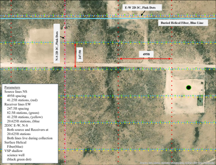
To test this idea, the field test layout (Figures 3a and 3b) was focused on super sampling the near-surface to image depths up to 4000ft with the focus on the first 250ft to 1500ft. For these shallow depths, the following spatial sampled tests with different receiver types were laid out. Source line spacing and source station spacing of 495ft X 41.25ft was the same for all receiver spacings listed.

• ● Geospace, 2816 geophones GSR 10Hz production survey: Receiver line spacing 495ft, stations 82.5ft, CDP bin 20.625ft X 41.25ft
• ● Inova, 11,008 geophones Quantum 5Hz: Receiver line spacing 247.5ft, stations 41.25ft, CDP bin 20.625ft X 20.625ft
• ● Stryde, 22,016 accelerometers: Receiver line spacing 247.5ft, stations 20.625ft, CDP bin 20.625ft X 10.3125ft
• ● The 4 square mile field test was sourced twice, first with a single vibe and again with the 3-vibe production survey. The receivers spatial sampling varied but co-location occurred at 82.5ft and 41.25ft. Therefore, the same source effort was used for each of the three 3D receiver surveys regardless of receiver type and spatial sampling. This allowed for detailed comparison of different receiver responses and different spatial sampling.
• ● The two 2D3C lines orthogonally laid out with Geospace GSX 10Hz 3C geophones. In this case, there was a 2-vibe source effort with source and receiver stations spaced at 20.625ft and CDP bin spacing of 10.3125ft.
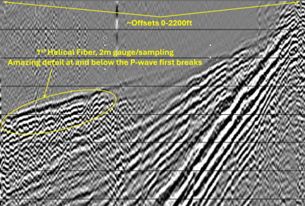
• ● A 4-fiber helical cable was buried on the surface, along 3000ft of the east-west 2D3C line. The 4 helical fibers recorded at 2, 5, and 10-meter gauge samplings (Hall, Lawton, & Innanen, 2022). The fiber data recorded all sources, including the sweep test, the 2D line 2-vibe acquisitions, and both the 1-vibe 3D and 3-vibe 3D acquisitions.

The second objective was to understand if seismic can be used to better illuminate the zones of interest below the fill zone and the required spatial sampling to achieve this goal. However, any differences between the receiver types and source efforts had to be accounted for before attributing the effects to spatial sampling.

The third seismic objective for comparing receiver types was to collect a broadband spectrum for quantitative interpretation. Therefore, the low-frequency response from each receiver type and the source effort to record low and high frequencies were part of the field tests.

A sweep test was performed to pick the production sweep. 37 different sweeps at 3 separate locations near the intersection of the two 2D3C seismic lines and the buried fiber were recorded. While evaluating the sweep tests, the two 2D3C N-S and E-W lines were acquired. The predetermined custom sweep for the 2D lines was 2-53Hz, 15 second long, and 6 seconds dwell in the 2-8Hz range using 2-vibes. The plan was to shoot the single vibe 3D with the same 2-53Hz sweep.

However, the fiber clearly showed sweeping higher to 72Hz or more, (Figure 4) had benefits to the shallow geology and first breaks. Therefore, once the production sweep was chosen, 2-84Hz, 24 seconds long, 6 seconds of dwell time, we used it in the single vibe 4 square mile 3D survey. When the production 3 vibes came back through, there was now a one-to-one comparison of the same sweep with different spatial receiver sampling, receiver types and a source effort of 1 versus 3 vibes.

Field Test Observations

All geophones and accelerometers performed well. Once the known phase and amplitude geophone response corrections between the 10Hz and 5Hz geophones were applied, raw records and stacks showed negligible differences.

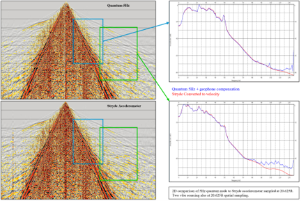
To compare velocity geophones to accelerometers, two workflows are available. The first is to allow the deconvolution operator to build the inverse filter to flatten the spectrum for the accelerometer data. Alternatively, acceleration data can be integrated and converted into velocity information, which allows similar processing to both geophone data and accelerometer data before and after deconvolution (Hons, Stewart, Lawton, & Bertram, 2007).

Past experience shows that in high signal-to-noise areas where low frequency source effort starts above 8Hz, deconvolution filters do a reasonable job of balancing the input source frequencies recorded. However, in very poor signal-to-noise areas such as the DB fill zone, converting acceleration to velocity is preferred for comparable results of field records and stacks (Figures 5a and 5b).

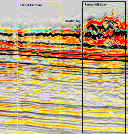
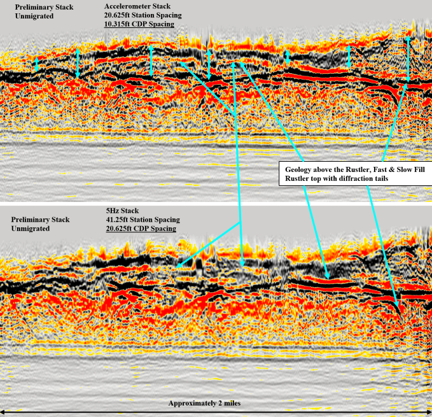
The primary observation is the fill tests illuminated the structurally complex Rustler formation (Figure 6). The complexity is due to the collapse of the halite in the Salado formation and halite benches in the Castile formation. This created two expanded weathering zones above the Rustler which have caused huge statics, scattering and coherent noise issues.

The Rustler formation structural complexity is the primary scatter point with hundreds of feet of vertical structure over a few hundred feet of lateral change. We then name two zones above the Rustler as the fast and slow fill. As it turns out, inability to resolve the statics and velocities through these two zones leads to an inability to image the Rustler and other geophysical challenges deeper in the section.

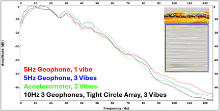
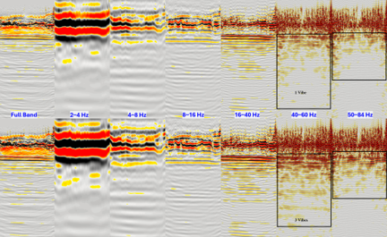
Another observation is that the 3-vibe acquisition is better than 1-vibe for the higher frequency bands above 40 hertz. In fact, an argument can be made that 3-vibes are better than 1 for all frequencies (Figure 7).

Conclusions

The primary goals of finding the top of the Rustler formation, building the correct velocity and static models represented by the near-surface geology, and imaging a broadband spectrum both under the fill and outside the fill, were achieved. The additional channels for spatial sampling provided the opportunity to compare 10Hz and 5Hz geophones with accelerometer receivers. With careful processing, all receivers showed similar response with negligible differences. Also, the need of 3-vibes versus 1-vibe was observed for broader bandwidth.

The second goal was to determine the value of the different spatial samplings. The production survey was the least dense at 41.25ft bin spacing but clearly sampled the top of the Rustler formation with some usable data in the fast and slow fill. However, the tighter receiver line, and station spacing with CDP binning of 20.625ft X 10.3125ft, showed great geologic detail in the shallowest fast and slow fill. The structurally complex Rustler top with the corresponding thickness and depth changes related to the fast and slow fill were captured in this test. That information was fed into resolution of large variable statics and the generation of a detailed near-surface velocity model. Therefore, quality depth imaging from the complex shallow surface geology, through the hydrocarbon zones of interest, and into the basement was achieved.

Acknowledgements

I would like to thank my colleagues and co-authors at Fairfield Geotechnologies, Dawson Geophysical for acquisition, Skyway Field Services, Stryde and Quantum for field equipment, Neubrex for fiber deployment and recording, Viridien for processing and the underwriters for making this a great collaboration.